|
Kyle Chuang | ME405 Mechatronics Portfolio
|


|
|
Kyle Chuang | ME405 Mechatronics Portfolio
|
|
In this lab, I worked with Enoch Nicholson to combine the motor and encoder driver from (Lab0x08: Term Project Part 1) and the touchscreen driver from (Lab0x07: Feeling Touchy) to balance a ball on our pivoting platform system. To implement this, we developed a proportional controller using the inputs of [xdot; thetadot_y; x; theta_y] via three methods: analytical solution, MATLAB simulation, and by implementing it into our hardware using Python.
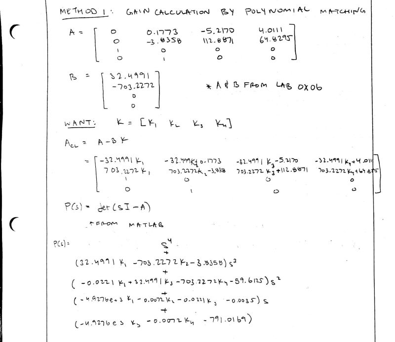
In this method, we found controller gains by characteristic polynomial matching. We started with our A and B matrices derived from (Lab0x06: Simulation or Reality?). For full state-feedback, the control input is defined as u = -K*x. We rewrote our state space system for our closed loop system as A_CL = A-BK, where K was represented by symbolic variables. Then, we found the characteristic polynomial for the system under closed loop feedback using P(s) = det(sI-A). The solution was done in matlab and can be seen in the image below.
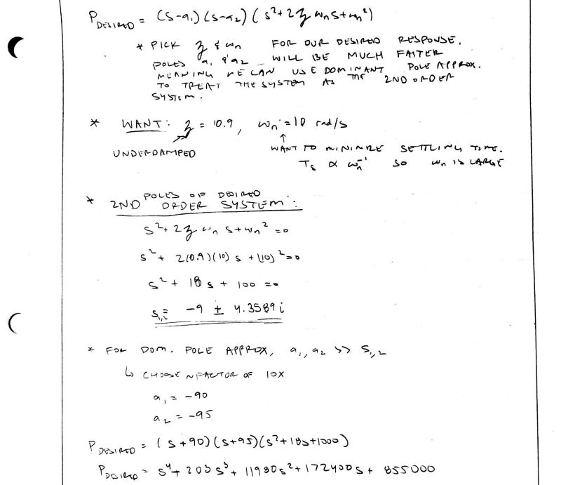
Next, we developed our desired model for the system. To do this, we selected our desired system qualities (zeta = 0.9 and w_n = 10 rad/s). We chose these parameters because our motors have some friction in its system and have trouble operating under low duty cycles. Thus, we decided that it would be better for the system to run faster and correct overshoot than it would be to run the system slower under lower duty cycles.
Once we had our desired system characteristics, we developed a second order system in accordance to these parameters and then found the poles. These will be our dominant poles that will govern our system. For this to happen, we needed to make our system a fourth order system with the same response as the second order system. We used the dominant pole approximation to make this happen, by placing the remaining two poles at least 10x larger than the real component of the poles from the second order system. The result is shown in the image below:
Lastly, we equated the coefficients of both polynomials and found our controller gains as K1 = -34.9901, K2 = -1.9112, K3 = -173.6941, and K4 = -25.1466. These gains were used as initial gain values for the hardware implementation. These values were verified using MATLAB's "place" command which resulted in controller gains of K1 = -34.9857, K2 = -1.9001, K3 = -173.6724, and K4 = -25.1456 for the poles -90, -95, -9+4.3589i, and -9-4.3589i.
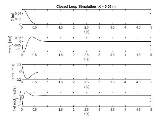
In this method, we found controller gains by modifying the simulation code from (Lab0x06: Simulation or Reality?) to solve for the K matrix. To do so, we used the linear-quadratic regulator MATLAB function (lqr) to set each input as a different priority. We prioritized the ball position over all other parameters because that is the goal of this project. Additionally, we put low priority on angular velocity to account for the motor friction. This resulted in controller gains of K1 = -9.6577, K2 = -0.8200, K3 = -31.7837, and K4 = -9.3184.
We plotted the result of this simulation for 5 seconds under the conditions of a flat plate and the ball offset by 0.05 meters.
In this method, we developed a main file (LINK TO MAIN) which implemented the basic functionality of a full state feedback controller (u = -K*x). In our case, x was our state vector consisting of [xdot; thetadot_y; x; theta_y], K was our gain matrix, and u was the torque input to the platform motors. To get ball position values, we used the touchscreen driver from (Lab0x07: Feeling Touchy) to obtain real-time inputs for x and y. To get theta values, we used the encoder driver from (Lab0x08: Term Project Part 1) to obtain real-time inputs for theta_x and theta_y. To get velocity values, we used change in position over change in time which completed our state space vector input. These values were multiplied by our gains to produce the required torque input for each motor. These were then converted to duty cycle values via a gain constant derived from the motor data sheet.
Because both Enoch and I wanted to get the full experience implementing this system, we each took a different, individual approach to making the ball balance.
Due to time constraints, I chose not to implement the BNO055 IMU sensor to automatically balance the platform. Instead, I designed the main file (balance.py) to have the user manually level the platform and input "0" on the keyboard to complete the leveling process. Then, the code will wait for an input to the touchscreen and respond according to the proportional controller gains. I tested the system iteratively by placing an emphasis on the inputs from the ball (x and xdot) starting with the gains found from the analytical and simulation methods and found that the gains of K1 = -100, K2 = -50, K3 = -500, and K4 = -20 demonstrate the trends of the expected response from the controller. These gains are far from the controller gains calculated in methods 1 and 2 most likely because of two reasons: unit errors in my code and the friciton involved in the motors which the controller must overcome in order to control the platform.
Still, my system is far from balancing the ball due to a number of reasons. For starters, the motor friction makes it difficult to implement fine movements for the ball. As a result, the motors overcompensate and the ball rolls right off. Additionally, my motor 1 has significant slack in the belt used to drive the output shaft. This causes the belt to skip when trying to drive the platform. On the software side of things, my code could be optimized to run faster as it currently is too slow to effectively balance the ball.
This video shows off the funcitonality (or lack thereof) of my system, and I summarize my design process for this controller:
In Enoch's approach, he chose to implement the BNO055 IMU to automatically balance the platform prior to the ball being placed on it. He also included a low pass, Finite Impulse Response filter to improve the inputs to our system. We followed a similar setup for our controllers, with his gains being K1 = -14.17333, K2_y = -14.4129, K2_x = -10.4129, K3 = -1.254464, and K4 = -0.00223331. (Note: Enoch's state space is set up differently from mine as his is [x; theta_y; xdot; thetadot_y]. Additionally, he tuned each motor gain separately which accounts for the two "K2" Values). His controller design is explained in greater detail in the documenation in his portfolio, but the performance of his system is highlighted in the video below.